Parallel inventory valuation – an alternative approach (Part 4)

07 Friday Apr 2017

Posted by Ludwig Reinhard in General Ledger, Inventory

≈ Comments Off on Parallel inventory valuation – an alternative approach (Part 4)

Tags

Inventory, lot size variance, parallel, standard costs, valuation

After the purchase and internal standard cost variances have been analyzed, let’s now have a look at the production related standard cost variances and how to deal with them.

Within this fourth part we will have a look at the lot size variance (LSV) first, which arises for example if the good quantity from a production order differs from the calculation quantity that was used for the standard cost calculation of an item. The following graphic illustrates the composition of the finished item that will be used for the subsequent explanations of the production lot size variance.

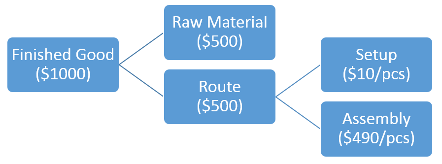
The graphic above shows a finished good that is made of a raw material that has a standard cost price of $500 setup. In addition, another $500 route related costs – that consist of $490 assembly cost and $10 setup cost – are necessary to produce the item.

As the setup costs are independent from the quantity produced, the total production costs of an item decrease, as the production quantity increases. The next graphic illustrates this relationship for the sample item used.

To illustrate how the lot size variance arises and how to deal with this kind of variance, a production order for 10 pcs of the finished good is processed. The next screen print shows that a total of $9910 production costs arise for the production of the 10 items [$10 setup costs + 10 x ($500 material costs + $490 assembly costs)]. The illustrated lot size variance of $90 results from the fix cost degression effect shown in the previous graphic.

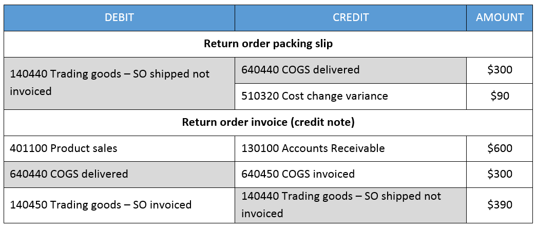
Similar to what has been shown in the previous post, the next accounting-like overview summarizes the production postings recorded (separated by the different production steps).

The grey highlighted lines offset each other and can thus be ignored for the analysis of the production costs.

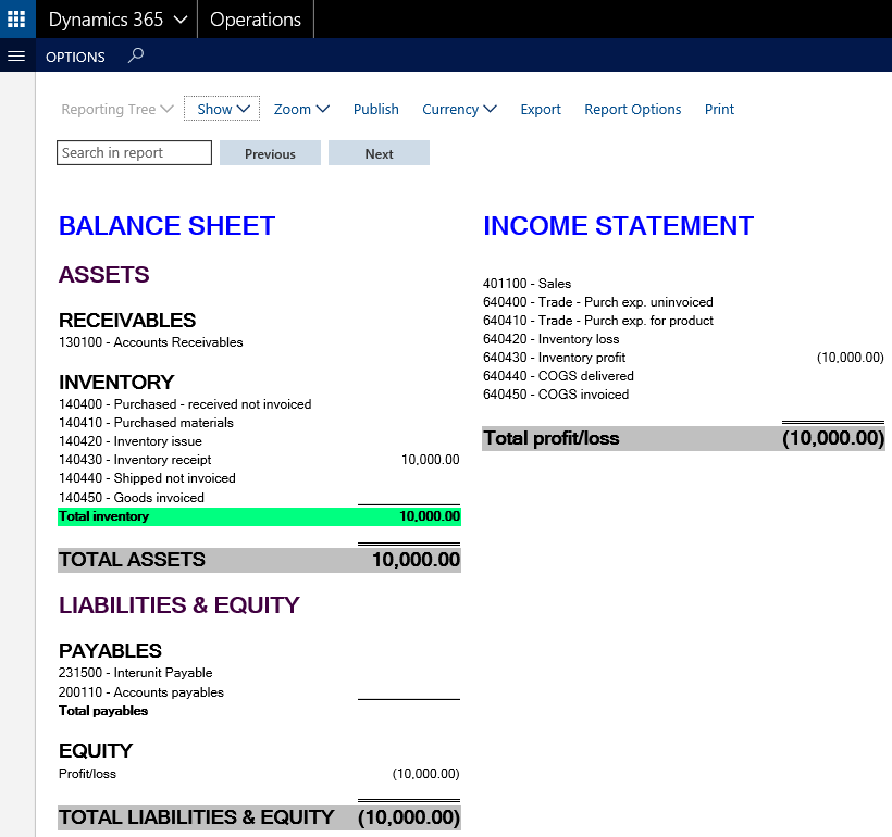
For those readers who are not very familiar with ledger postings, the following financial statement overview has been prepared.

The financial statement overview shows a total inventory value of $10000 for the finished product on ledger account 140670. To produce those finished goods, raw materials with a total value of $5000 and $4910 labor costs have been consumed. The remaining difference to the standard cost value of the finished goods is assigned to the lot size variance that is recorded on ledger account 540630.

Further above, a realized cost amount of $9910 has been identified. Against the background of this actual cost amount, it can be concluded that the inventory value of the finished goods is overstated by $90 from an actual costing perspective.

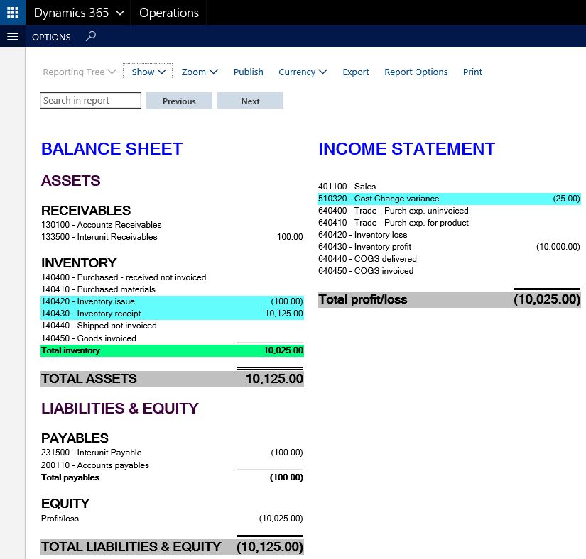
If one of the produced items is sold later on, the inventory value is decreased by $1000 – the standard costs of the item. The financial statements illustrated below exemplifies this situation.

From an actual costing perspective, the decrease in the inventory value from the sale of the produced item is comparatively too high. The same holds for the cost of sales, which are recorded on ledger account 640650.

In order to arrive at an actual cost valuation, the lot size variance (LSV) needs consequently be adjusted and split up in a similar way that has been shown for the purchase price variance before. The next graphic exemplifies the necessary separation of the total lot size variance if one out of the ten produced items is sold.

To conserve space, the setup of the necessary ledger allocation rule is left as an exercise for the reader. If the allocation rule is later on processed, the following financial statements result:

The financial statement overview shows a total inventory value that is $81 lower than before. This reduction takes care of the difference between the actual and the standard cost price [9 pcs x ($1000 – $991)]. As the allocated lot size variance amount is recorded on a separate ledger account, a parallel standard cost and actual cost inventory valuation can be achieved.

Please note that this also applies for the COGS amount of $1000 that has been adjusted through a corresponding adjustment on ledger account 640651 to arrive at an actual cost value of $991.

Within the next post we will take a look at the other production related standard cost variances and how to deal with them from a parallel valuation perspective. Till then.

Parallel inventory valuation – an alternative approach (Part 3)

28 Tuesday Mar 2017

Posted by Ludwig Reinhard in General Ledger, Inventory

≈ 2 Comments

Tags

cost change variance, Inventory, parallel, standard costs, valuation

The next standard cost variance type that has an influence on the parallel valuation approach concerns cost change variances, which can result from two different sources that will be explained in the following.

Source 1: Standard cost price differences between sites
Standard costs can be setup in a way that different standard cost prices are defined per site in order to incorporate cost price differences resulting for example from transportation costs, etc. The next screen print exemplifies an item that has different cost prices setup for site 1 and site 2.

In order to illustrate what influence these different cost prices have on the parallel inventory valuation approach, 100 pcs of the item have initially been acquired through an inventory adjustment journal for site 1. The resulting financial data can be identified in the following screen print.

After the items have been acquired, an inventory transfer from site 1 to site 2 for a single item is posted through an inventory transfer journal.

The outcome of this transfer is an adjustment voucher that results in a corresponding increase in the inventory value. The adjustment voucher and the resulting inventory value increase can be identified in the following figures.

What one can identify from the financial statement reports exemplified above is that the total inventory value increased by $25 because of the item transfer from site 1 to site 2.

Before analyzing how to deal with that variance for the parallel inventory valuation approach, let’s have a look at the second possible source of cost change variances.

Source 2: Customer item return after standard cost price change

A second possible source for cost change variances are situations where standard cost items are sold to customers and returned after a cost price adjustment has been completed.

The following example illustrates this scenario where initially 100 pcs of a standard cost item with a cost price of $100/pcs are acquired – for reasons of simplicity – through an inventory adjustment journal. The next screen print shows the resulting financial statements.

After the items have been acquired, 5 pcs are sold for a sales price of $200/pcs. With a standard cost price of $100/pcs, the company’s inventory value is consequently reduced by $500, which can be identified from the next financial statement illustration.

Shortly after the items have been sold, the standard cost price of the remaining inventory items is adjusted from $100 to $130. The resulting accounting voucher and financial statements are shown in the next screen prints.

The screen prints above illustrate that the change in the standard cost price resulted in a $2850 higher inventory value [95 pieces x ($130-$100)].

After the standard cost price has been increased from $100 to $130, the customer decided to return 3 out of the 5 pcs sold. Posting the return order packing slip and invoice results in a number of transaction vouchers that are summarized in the next accounting-like overview.

The grey highlighted lines offset each other and can thus be ignored for the analysis of the production costs.

The transaction vouchers summarized above demonstrate that the item return resulted in a corresponding adjustment of the sales revenue and the receivables amount (3 pcs x $200 sales price / pcs = $600). At the same time, an adjustment of the COGS and inventory value was recorded. Yet, because of the cost price change, a $90 higher inventory value remains.

Expressed differently, selling and returning the 3 items resulted in a $90 higher inventory value, which can be identified in the following financial statement overview.

After having analyzed the sources of cost change variances, the question arises, how to deal with them in order to arrive at a parallel actual cost based inventory value?

As mentioned in the previous post, standard cost price changes resp. differences typically do not reflect actual (market) price differences but rather cost/transportation/handling cost differences.

Moreover, in an actual inventory costing environment, internal movements of goods between different sites do not affect the company’s profit. That is, a company does not get richer or poorer by the mere fact that an item has been shifted from one location to the other, as it might be the case for standard cost items.

The same holds for the second source of the identified cost price changes; i.e. in an actual costing environment, a company does not get richer or poorer by shipping and returning goods to and from a customer, as it might be the case in a standard cost environment.

For those reasons and because cost change variances affect receipt transactions only, it can be argued that the complete cost change variance amount needs to be shifted from the company’s income statement to it’s balance sheet in order to arrive at an approximate actual cost valuation. This shifting can once again be realized by making use on an allocation rule similar to the one that has been introduced in the prior posts.

The next posts will deal with the production related standard cost variances and how to incorporate them in the parallel inventory valuation approach. Till then.

Parallel inventory valuation – an alternative approach (Part 2)

15 Wednesday Mar 2017

Posted by Ludwig Reinhard in General Ledger, Inventory

≈ Comments Off on Parallel inventory valuation – an alternative approach (Part 2)

Tags

Inventory, inventory cost revaluation, parallel, standard costs, valuation

After having analyzed how to deal with purchase price variances in order to arrive at a second (parallel) inventory value, let’s have a look at the second standard cost variance type – the inventory cost revaluation – and how to deal with those variances to obtain a second (parallel) inventory value for standard cost items.

Scenario:
At the end of a fiscal year, the standard costs of a first item are adjusted from $100 to $109. For a second standard cost item, the standard costs are adjusted from $100 to $95. As there are currently 100 pcs from each of the items on stock, a total inventory value of $20000 can be identified (before adjusting the standard cost prices) in the financial statements illustrated in the next figure.

For reasons of simplicity the inventory values/balances have been created by posting an inventory adjustment journal that resulted in an inventory receipt & profit transaction.

The aforementioned revaluation of the standard cost item is realized by recording and activating the new standard cost prices in the standard cost costing version, as exemplified in the next screen print.

Once the new standard cost prices are activated, the financial statements show a $400 higher inventory value. This can be identified from the next figure.

The overall increase in the inventory value can be explained by the value increase of the first standard cost item [($109-$100) x 100 pcs] and the value decrease of the second standard cost item [($95-$100) x 100 pcs]. If the revalued items will be sold subsequently, the newly activated standard cost prices will be used for posting the issue transactions.

At this point the question arises whether the inventory cost revaluation amount can remain in the income statement as illustrated in the previous screen print or whether an adjustment similar to the one that has been shown in the first part for the purchase price variance (PPV) is required in order to get a second (parallel) inventory value?

This question can be answered by stating that no split and allocation of the cost revaluation is required, if the cost revaluation is done in a way to adjust the standard cost prices to an ‘actual’ market price. If this is the case, any previously recorded adjustment and allocation of the PPV needs to be reversed in order to avoid an over-adjustment of inventory values towards actual market prices/values.

In practice, most companies do not adjust their standard cost prices in a way to reflect ‘actual’ (market) cost prices. Otherwise, they would have chosen an alternative actual cost price valuation model right from the beginning. Against the background of this common adjustment behavior, it can be argued that an adjustment of the recorded standard cost revaluation amount is necessary in order to arrive at an approximated actual inventory cost price. The main question in this context is then how such an adjustment can be realized?

From the authors’ perspective, the complete cost revaluation amount needs to be shifted (allocated) from the income statement to the balance sheet in order to arrive at an actual cost valuation amount. That is because only those items that are currently on stock (or in process) – that is receipt transactions – are affected by the cost change variance. If those items are sold or consumed later on the adjusted higher/lower standard cost price will ensure that the cost revaluation amount that has been allocated to the balance sheet is successively eliminated. For that reason no split up and allocation of the cost revaluation amount is necessary.

The next part of this series continues with analyzing cost change variances and how they need to be incorporated into this parallel inventory valuation approach.